Vector graphics editor software are SUPER useful when trying to make figures. A proprietary program some people may be used to is Adobe Illustrator. I’ve never actually used it, mostly b/c I started using playing around with vector graphics editor software when I was a grad student, and the idea of paying for an Adobe product with my own money was unpalatable. Inkscape is a free & open source software that works on Mac or Windows. It can be a little buggy, but I’ve learned to absolutely love it over the last 10 years or so. To help people in my lab start using it, I’m writing up this primer describing a series of basic processes I perform when using it.

Step 1: Downloading Inkscape. Obviously, this is downloading the program. I’ll assume this is pretty self-explanatory unless someone tells me otherwise.

Step 2: Starting up the program. You should get a blank screen like this, which is the basic workspace. The white rectangle with the drop-shadow is the blank “page”.

Step 3: Adjusting the properties of your page. While you don’t have to start here, I like to make some basic adjustments to the page out of the get-go. To do this, go to File -> Document Properties… or just hit “Command + Shift + D” if you’re on a Mac, like me. A new pane should open up to the right of the program, like below (if it doesn’t, try adjusting the size of your window and that should force a refresh).

The main things I like to change are as follows:
1) The dimensions. Most journal have maximum figure widths between 174 and 180 mm (though handful allow 190 or even 200 mm). It’s probably easier to plan for the smallest size of 174 mm, and just space things apart a bit / give the panels more breathing room if you end up in a situation where larger dimensions are allowed. Thus, adjust the width to 174 mm, and hit enter, and the width of that page should now shrink.
2) So the page settings defaults to *NO* background color (this can be revealed by clicking on that “Checkerboard background” button). So if you put in some shapes / plots, they will be floating in emptiness, rather than a white background. While this isn’t problematic per-se, it usually makes sense to make figures that actually have a white background. Thus, I next click on that box next to the text that says “Background color:” and in the bottom field that has a 0 next to “A:”, I change that to 100 (I’m assuming this is opacity, and we are turning the opacity from 0 to 100). This will make the background white.

Step 3: Saving the file. Now that you’ve made some modifications to your file, you may as well save it (since you’re going to want to start saving the file soon anyway). Go to File -> Save As… and save the file in whatever directory you want to keep it. The file type is will save is a “.svg” file, apparently for an “Inkscape svg” file, which is seemingly a slight derivation of a pretty genetic / standard file type for vector graphics (svg). You can just keep these default settings.

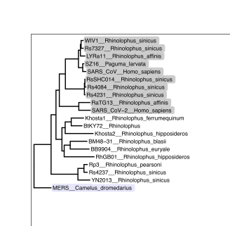
Step 4: Import some existing vector graphics data. So while you can start from scratch making shapes in the program itself, I’m most often using Inkscape to make adjustments to vector graphics plots generated in another program, like R. In this case, I’ll be importing a phylogenetic tree based on the spike protein receptor binding domain sequences from various coronaviruses. Thus, go to File -> Import… or hit “Command + I”, or press that arrow-point-to-a-page button at the top of the screen, to prompt the import screen,.

In the ensuing screen, point to the file you’re trying to import. If it’s a vector graphics -compatible file, then this will most likely be a “.pdf” type file. After you select a file, you’ll get a screen like this:

You can probably just click “OK”, since I’ve found these default settings to generally work fine. All of the shapes will all get imported fine, though I’ve found that the text gets imported kind of weird. Like, the letters are fine if you don’t make any adjustments, but if you try to rewrite any of the letters, you’ll notice that the spacing gets all screwed up. I usually just get around that by replacing the imported text with replacement text that I’ve created using Inkscape, though that gets a bit tedious. I suppose maybe one day I’ll learn if there is a better way to import text from a PDF, but for now, this will do.

Step 5: Adjust the positions and sizes of things. Depending on the dimensions of your image as it was outputted by the preceding program (like R), your image may or may not fit well within your blank page. In my case here, the image was indeed roughly the right size, though I wanted to zoom in a bit to see it in a bit more detail. To do this, I pressed the “+” button my keyboard a couple of times to get to the desired zoom, though you can adjust the Zoom in more detail on the bottom right of the screen (see below):

Another thing you may want to do is adjust the size and position of the image / plot you just imported. If you want to keep everything in the right dimensions, the first thing you’ll want to do is click on the “lock” button making sure the height and width stay in proportion.

Then you can type in whatever number you want into either the W: or H: fields, hit enter, and see if the size was adjusted to what you’d like. Another thing that’s useful is to adjust the position of the image. For example, perhaps this is the first panel of your figure, and you want it in the top left of the page. If that’s the case, enter 0 for both the X: and Y: fields, and hit enter (In many cases, you’ll want at least a couple pixels worth of blank space around the borders, in which case typing in something like 2 is better, but I’m using 0 today to prove a later point). Now the plot should look like so:

Step 6: Ungrouping and adjusting vector objects. As you can see, the border is now missing. Why is that? Well, it’s because in this case, the phylogenetic tree pdf I imported also had a white background, so that white background is now obstructing the borders of the page under it. While this isn’t necessarily problematic, this extra white background is superfluous and may complicate things downstream, so we will now get rid of it. To do so, click on the object, and go to Object -> Ungroup, or just hit the “Command + U” keys like I do. That one object should now have been turned into a bunch of objects, each with its own highlighting, showing that the ungroup command worked.

Unselect everything, and then select only the white background. Once you seem to have selected it, hit delete. If you missed and you deleted the wrong thing, you can undo. If you’re having a hard time selecting the white background because there is something in the foreground that inevitably gets selected first, you can take that foreground element and then hit the “send to back” button at the top of the screen to get that foreground element out of the way.

Once you do that, you should be able to more easily select the background element and hit delete. (In this case, there were apparently two background elements I had to individually select and delete). The end result should now look like this, where you can now see the Inkscape “page” borders again.

Once you do that, the start and end points of each of those lines are now selectable. Since I want to adjust both lines on the left size (and make it smaller by moving them to the right), click on one of those points, and then Shift-Click on the other point. If they’re both selected, they should look different from the points on the right side of the line.

Once they’re selected, you can move them to the right. I like to do fine manipulating at this scale using the arrow keys on the keyboard. So, I *could* hit the right arrow to move those nodes to the right and thus shortening the lines. Then again, I’d probably have to hit that button ~ 100 times to move it to the right the amount I want. That’s b/c by default, the arrows are “fine” adjustments. To turn the arrows into “coarse” adjustments, hold down the shift key as you press the arrow buttons. I only had to hit “Shift + [Right Arrow]” four times to get those lines to the length I wanted them.

That worked well, but now that connecting line is orphaned and confusing. We can now move that to the right by selecting that, and since we’re not selecting individual nodes but just moving the entire line itself, we can hit “Shift + [Right Arrow]” four times *without* first hitting that “Edit paths by nodes” button. If you already have the “Edit paths by nodes” button enabled (and thus shaded gray), you may need to turn it into the other “Select and transform objects” mode by clicking on the button above the “Edit paths by nodes” button. I’m also now moving everything to the left by selecting everything and entering X: 1 and Y: 1 as I mentioned above. It should now look like so:

Progress! Though adjusting the tree like we did can be disingenuous, since both the adjust lines we shorted (for the outgroup) is the same color & texture as the lines we didn’t adjust (for the rest of the tree). To distinguish between the two, we can click on the lines leading to the outgroup and change its style / texture to a dotted or interval one. That way, we can write in the figure legend later on that the dotted lines leading to the outgroup were adjusted to conserve figure space. To do this, click on the lines in question (holding down shift while doing so, so that all four individual lines can be selected), and then hit the color / button associated with the “Stroke:” label at the very bottom-left of your screen (see orange highlighted circle in the image below). This should open up a new page to the right. If you still have the “Document Properties” pane open from before, you may need to close it out (by hitting the “X” button at the top right of that pane), or just scroll down until you get to the “Fill and Stroke” pane. Apparently one can also get to this pane by hitting “Command + Shift + F”.

While you still have those lines selected, you can click on the tab that says “Stroke style” and then go to the button that says Dashes, and click on a style that has dots or dashes. You may also need to adjust the width of the line, so that it’s a bit more pronounced (I set it to 1 pixel).

The end result should look like this. A much better use of space!

Since this is potentially panel A, let’s make a panel label. To do this, click on the button labeled with “A” on the left side (the “Create and edit text objects” button), and then *drag* a text box roughly in the right area of where you’ll want it. Note: While you can *click* and make a test object, dragging is better because then you can modify the size of that text object later (less relevant for things like figure labels, but *definitely* important for things like figure legends). In this case, I typed in the letter “A”, turned it into bold. Once I did that, I clicked on the now bolded A, and then adjusted the X: and Y: to 1 so it’s now in the top left corner, like so:

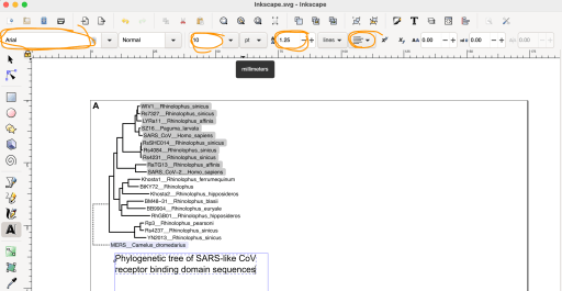
Step 8: Aligning some object together. OK, well this figure doesn’t actually need this label, but let’s pretend we want to make a short one-line label / title at the bottom, and we want it right at the center of the tree. Make a text box like before, and type in your label. If you select the text box and are in text editing mode (you may need to click on the “A” button on the left again), you have the option to change fonts, bold / italics, size, line spacing, and line justification / centering in a series of boxes at the top. The one I adjust ALL the time is the line spacing. It defaults to 1.25, but it’s kind of waste of space like that, so I set it to 1.

Once you’ve done all that, you should have a screen that looks like below:

This pane will allow you to align things based on the right edge, left edge, the center. Or if you have multiple objects that you want to space equally, you can go to the Distribute button options in the middle. Looks like it’s defaulted to “Relative to: Last selected”. That means that if you’re aligning two objects, the object you select first will be moved to the objected you selected second. You can of course change that order if you change the “Relative to:” to “First selected”. But in this case, I’m leaving it as the default, so I first selected the legend, and then selected the tree, and then hit the “Center by Vertical Axis” button that I highlighted in orange. The resulting image looks like this, where now the elements are aligned!

Step 9: Exporting your image. OK, so I’ve done everything I’ve wanted to do for this tutorial, so that last thing will be exporting the image. You have two options here. You can make a PDF that can be imported into whatever program later, by going to File -> Save As… and then instead of saving it as a .svg file, saving it as a .pdf file. (Note: this will change the workspace you’re working in to be a “.pdf”. If you want to have the workspace be an “.svg”, you’ll need to resave into that format. Or if you don’t want to do this roundabout process, you can also do File -> Print, and then select “Print to File”; all this is up to you). But, let’s pretend you want to actually submit this as a figure for a manuscript submission. Usually the desired filetype is as an image file rather than a vector graphic. This means something like an uncompressed .tif or .png file (instead of a compressed .jpg file). To do this, click on File -> Export PNG Image… , or click on the “Arrow coming out of page” button next to the import button at the top of the screen. This will open up another pane to the right:

For novices, I suggest you always click on “Page” for the Export area; this means it will export that full canvas you have been looking at (with the full width of 174 mm or whatever you had set before), rather than just the selected object, etc. You can adjust the dots per inch or DPI, but the default 300 is usually pretty good. And of course, you can and should change where the file is being saved. Once you do that, hit the “Export” button on the bottom. A little pop-up screen will show the export process (should be relatively quick for files like this). And Voila! You’ve made yourself a nice little customized image!

Update 1: Now with Western Blots.
I told myself that I would document the next time I was going to insert some image files into Inkscape for the purposes of this post, and here we are. So let’s now set the scene:

OK, so we have a multi-panel figure in the works here. The only panel relevant to today’s post is panel B, which is going to be a couple of Western Blotting images. In short, we have a negative control lysate, as well as 5 experimental samples where a different protein has been HA-tagged in each lysate. Looks like the first 3 proteins express quite highly, while the last two are expressed at pretty low levels. Thus, I’m going to try putting a lighter exposure image on the left side, and probably a cropped right portion of a longer exposure image showing the last few samples to the right.

Well, first thing to do is press that import button (circled in orange) at the top of the page. Doing that will open up a window like below, where you’ll want to select the image you want to import into your canvas.

Once you choose a file, you should get another screen like the one below. Default settings are fine in my experience, so you can just hit “OK”.

Do this for all of the images you may want. The image files, if they are of pretty normal quality, will be imported as HUGE dimensions on the canvas. Reduce the dimensions of the file to something more reasonable, like 150 pixels. You’ll see yourself in a situation like this:

Now to start aligning the images, the main trick you’ll to using today is “setting a clip”. In other words, instead of cropping the edges off of an image like one would normally do in Powerpoint, you instead make an area that you save from being cropped. Thus, to do this, I start by making a partially transparent box above the relevant bands, like these actin bands here.

Doing so reduces the bottom image to the size of the top object. So now it’s the Blot image that has effectively been cropped.

Well, so I didn’t do a great job centering this crop, so I went back and fixed it but didn’t bother to retake the images. But if you’re curious, you can actually do this by right clicking on the object and hitting “Release Clip” to turn them into two separate objects again. Then just resize the box, select everything again, and then right click and hit “Set Clip” again.

Alright; now we can get one of the other exposures cropped and lined up. So now, I’ve moved in one of the other exposures in proximity to the red box. Since I’m going to have to make a larger field of view for this cropping, how straight the image is lined up is going to matter a lot more. For that reason, I drew in a black vertical line to visually inspect how straight it all seems. For the most part looks pretty good.

Allright, so I don’t need that line anymore so I went ahead and deleted it. But as I had mentioned; I want to get a larger window of the blot as compared to actin (a single horizontal band). Thus, I want to keep the width of the box the same but change the height of the box. To do this, click on the image, and you’ll see it have these arrows coming out of it.

Well, just click on the top and bottom arrows and drag to the height that you want it. It should now look something like this.

I can then crop and get the most relevant part of the image. Now that I have the cropped image, I can now align the two images together.

Now move everything in place. If you have another image, like a darker exposure, then you can just go back and repeat some of the previous steps for that one. You can even give them an outline, by duplicating the image, releasing the clip, deleting the repeated image, but turning hte red box into a completely clear box with a solid stroke; essentially, turning it into a see-through frame. Anyway, at this point, you should have a plot like above.

Next, making a bunch of labels to denote what each sample is. You can do that by dragging a text box, and then typing in your label. Once you’ve written the text you want for the first columns, duplicate that text box and replace the existing text with the text for the next sample, and keep doing this until everything is correctly labeled. When trying to make row labels, you may encounter needing to get some special greek characters like I did. In that case, while in the text box, go to Text -> Unicode Characters… and select it (see below).

You’ll get a box that looks like below, where you’ll want to click and select “Greek and Coptic”.

End result after you finish fixing the text should look like so:

Last bit is adding in the size labels, at least for the blot in the middle, since it spans a pretty large size. Alright, well, how would I go about doing this? Well, it’s pretty easy for the imager that we use, since it seems to spit out a combined image of the marker and the exposure, into a file that looks like this when imported into Inkscape (and resized to be the same dimensions of the lower exposure blot from earlier, and aligned on the vertical axis); here they are side-by-side.

If you want to prove to yourself that they are perfectly aligned, you can click both the actual lower exposure image and the marker-exposure overlay image, align them on both the vertical and horizontal axis, and then toggle the order back and forth (make the top image the bottom, and them make the bottom image top, etc). I did this, and they indeed seem to be perfectly aligned / superimposable (as one would expect). So knowing this, I’ll move forward by leaving tick marks where each of those marker labels are. Looks like the ladder we used is this one from GenScript.

Cool, now I can delete the overlaid picture, reset the clip on the original low exposure image, and then move the marker labels to a convenient spot to the left. Voila! (see below).

Additional resources:
I haven’t vetted this tutorial page, but it looks like it could potentially be useful.